深入了解Faster R-CNN实现细节

代码层面了解Faster R-CNN的实现细节, 重点RPN以及ROI pooling

前言

Faster R-CNN首次提出了anchor,使用RPN网络快速提取proposals,取代了耗时的selective search方法,大大提高检测效率.
Faster R-CNN的anchor思想被用于之后的YOLO和SSD等检测算法
关于Faster R-CNN的实现细节在下面的博客中已经做了介绍,本文主要从中抽取一些重点便于后面的回顾。
[Faster R-CNN基于代码实现的细节]https://blog.csdn.net/williamyi96/article/details/77648047

Faster R-CNN的基本结构

"da"

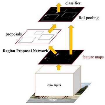
Faster R-CNN主要分为四个部分:
1.Conv layers. 使用一组基础的conv+relu+pooling层提取image的feature maps.

2.Region Proposal Networks. 该层生成一系列anchors并映射到原图,然后通过softmax判断anchors属于foreground或者background,再利用bounding box regression修正anchors获得精确的proposals.

3.Roi Pooling. 该层收集输入的feature maps和proposals,综合这些信息后提取proposal feature,送入后续全连接层判定目标类别.

4.Classification. 利用proposal feature maps计算proposal的类别,同时再次bounding box regression获得检测框最终的精确位置.

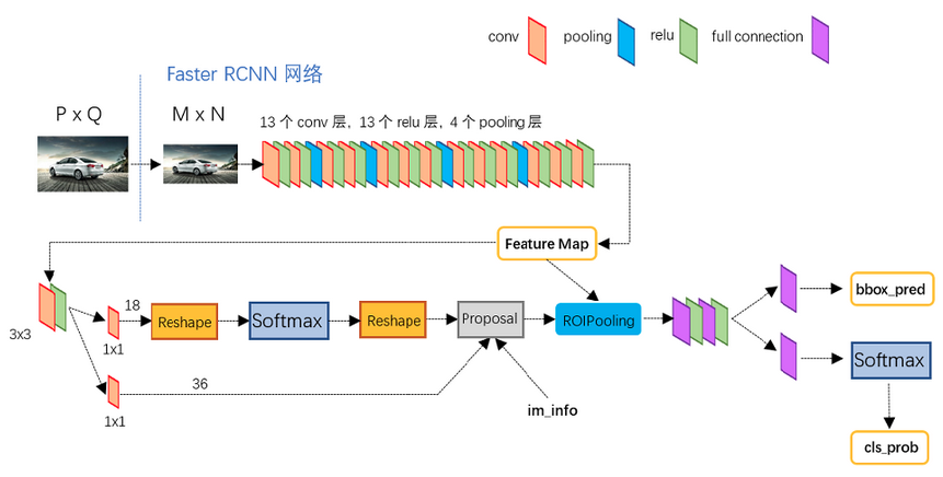
下图展示了Python版本中的VGG16模型中的faster_rcnn_test.pt的网络结构

"da"

Conv layers

Conv layers部分共有13个conv层,13个relu层,4个pooling层
为保证Conv layers生成的featuure map中都可以和原图对应起来, 卷积过程中使用pad保证卷积后宽高不变, 经过一次pooling操作, 宽高变为原来的1/2.
一个MxN大小的矩阵经过Conv layers固定变为(M/16)x(N/16).

RPN

RPN网络结构如下图所示

"da"

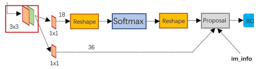
RPN网络实际分为2条线,上面一条通过softmax分类anchors获得foreground和background(检测目标是foreground),下面一条用于计算对于anchors的bounding box regression偏移量,以获得精确的proposal。
最后的Proposal层则负责综合foreground anchors和bounding box regression偏移量获取proposals,同时剔除太小和超出边界的proposals。
其实整个网络到了Proposal Layer这里,就完成了相当于目标定位的功能。

anchors

借用Faster RCNN论文中的原图,如下图,遍历Conv layers计算获得的feature maps,为每一个点都配备这9种anchors作为初始的检测框,后续通过边框回归可以修正检测框位置.

"da"

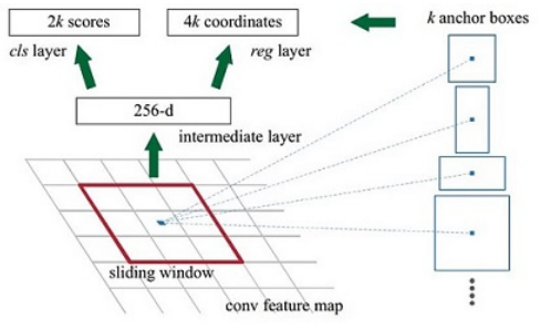
1.在原文中使用的是ZF model中,其Conv Layers中最后的conv5层num_output=256,对应生成256张特征图,所以相当于feature map每个点都是256-d
2.rpn_conv/3x3卷积后,相当于每个点又融合了周围3x3的空间信息
3.假设在conv5 feature map中每个点上有k个anchor(默认k=9),而每个anhcor要分foreground和background,所以每个点由256d feature转化为cls=2k scores;而每个anchor都有[x, y, w, h]对应4个偏移量,所以reg=4k coordinates

softmax判定foreground与background

在进入reshape与softmax之前,先做了1x1卷积

"da"

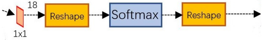
该1x1卷积的caffe prototxt定义如下:

1
2
3
4
5
6
7
8
9
10
layer {
name: "rpn_cls_score"
type: "Convolution"
bottom: "rpn/output"
top: "rpn_cls_score"
convolution_param {
num_output: 18 # 2(bg/fg) * 9(anchors)
kernel_size: 1 pad: 0 stride: 1
}
}

该层输出:WxHx18
feature maps每一个点都有9个anchors,同时每个anchors又有可能是foreground和background
相当于初步提取了检测目标候选区域box(一般认为目标在foreground anchors中)

在softmax前后都接一个reshape layer目的是为了便于softmax分类
在caffe基本数据结构blob中以如下形式保存数据:
blob=[batch_size, channel,height,width]
对应至上面的保存bg/fg anchors的矩阵,其在caffe blob中的存储形式为[1, 2*9, H, W]。

而在softmax分类时需要进行fg/bg二分类,所以reshape layer会将其变为[1, 2, 9*H, W]大小,即单独“腾空”出来一个维度以便softmax分类,之后再reshape回复原状。

caffe softmax_loss_layer.cpp的reshape函数的解释:

1
2
3
4
"Number of labels must match number of predictions; "
"e.g., if softmax axis == 1 and prediction shape is (N, C, H, W), "
"label count (number of labels) must be N*H*W, "
"with integer values in {0, 1, ..., C-1}.";

综上所述,RPN网络中利用anchors和softmax初步提取出foreground anchors作为候选区域。

边框回归

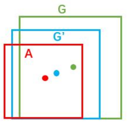
如下图,给定anchor A=(Ax, Ay, Aw, Ah),GT=[Gx, Gy, Gw, Gh],寻找一种变换F:使得F(Ax, Ay, Aw, Ah)=(G’x, G’y, G’w, G’h),其中(G’x, G’y, G’w, G’h)≈(Gx, Gy, Gw, Gh)。
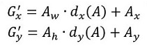
"da"

变换F的思路一般就是先做平移

"da"

再做缩放

"da"

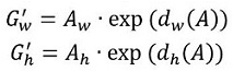
需要学习的是dx(A),dy(A),dw(A),dh(A)这四个变换

论文中的描述如下

"da"

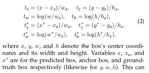
接下来就是如何通过线性回归获得dx(A),dy(A),dw(A),dh(A)了(即tx,ty,tw,th)。

线性回归就是给定输入的特征向量X, 学习一组参数W, 使得经过线性回归后的值跟真实值Y非常接近,即Y=WX。
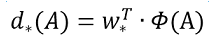
对于该问题,输入X是一张经过卷积获得的feature map,定义为Φ;同时还有训练传入的GT,即(gx, gy, gw, gh)。输出是dx(A),dy(A),dw(A),dh(A)四个变换。那么目标函数可以表示为:
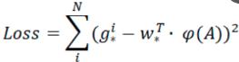
"da"

损失函数计算如下

"da"

对proposals进行bounding box regression

来看RPN网络第二条线路

"da"

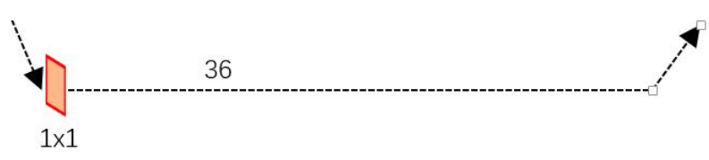
先来看一看上图中1x1卷积的caffe prototxt定义

1
2
3
4
5
6
7
8
9
10
layer {
name: "rpn_bbox_pred"
type: "Convolution"
bottom: "rpn/output"
top: "rpn_bbox_pred"
convolution_param {
num_output: 36 # 4 * 9(anchors)
kernel_size: 1 pad: 0 stride: 1
}
}

可以看到其num_output=36,即经过该卷积输出图像为WxHx36,在caffe blob存储为[1, 36, H, W],这里相当于feature maps每个点都有9个anchors,每个anchors又都有4个用于回归的[dx(A),dy(A),dw(A),dh(A)]变换量

Proposal Layer

Proposal Layer负责综合所有[dx(A),dy(A),dw(A),dh(A)]变换量和foreground anchors,计算出精准的proposal,送入后续RoI Pooling Layer。
Proposal Layer的caffe prototxt定义如下:

1
2
3
4
5
6
7
8
9
10
11
12
13
layer {
name: 'proposal'
type: 'Python'
bottom: 'rpn_cls_prob_reshape'
bottom: 'rpn_bbox_pred'
bottom: 'im_info'
top: 'rois'
python_param {
module: 'rpn.proposal_layer'
layer: 'ProposalLayer'
param_str: "'feat_stride': 16"
}
}

Proposal Layer有3个输入:
fg/bg anchors分类器结果rpn_cls_prob_reshape,
对应的bbox reg的[dx(A),dy(A),dw(A),dh(A)]变换量rpn_bbox_pred,以及im_info;
另外还有参数feat_stride=16,指的是四次pooling后map缩小为1/16。

Proposal Layer网络的前向过程大致如下:
1.生成anchors ,利用[dx(A),dy(A),dw(A),dh(A)]对所有的anchors做bbox regression回归

注意这里才生成anchors,即生成在原图中anchors的坐标
2.按照输入的foreground softmax scores由大到小排序anchors,提取前pre_nms_topN(e.g. 6000)个anchors,即提取修正位置后的foreground anchors。

3.利用im_info将fg anchors从MxN尺度映射回PxQ原图,判断fg anchors是否大范围超过边界,剔除严重超出边界fg anchors

4.进行nms

5.再次按照nms后的foreground softmax scores由大到小排序fg anchors,提取前post_nms_topN(e.g. 300)结果作为proposal输出

ROI pooling

RoI Pooling层负责收集proposal,统一proposals的尺度,送入后续网络。从图2中可以看到Rol pooling层有2个输入
1.原始的feature maps
2.RPN输出的proposal boxes(大小各不相同)

1
2
3
4
5
6
7
8
9
10
11
12
layer {
name: "roi_pool5"
type: "ROIPooling"
bottom: "conv5_3"
bottom: "rois"
top: "pool5"
roi_pooling_param {
pooled_w: 7
pooled_h: 7
spatial_scale: 0.0625 # 1/16
}
}

下面来研究一下caffe的具体实现

1
2
3
4
5
6
7
8
9
10
11
12
13
14
15
16
17
18
19
20
21
22
23
24
25
26
27
28
29
30
31
32
33
34
35
36
37
38
39
40
41
42
43
44
45
46
47
48
49
50
51
52
53
54
55
56
57
58
59
60
61
62
63
64
65
66
67
68
69
70
71
72
73
74
75
76
77
78
79
80
81
82
83
84
85
86
87
88
89
90
91
92
93
94
95
96
97
98
99
100
101
102
103
104
105
106
107
108
109
110
111
112
113
114
115
116
117
118
119
120
121
122
123
124
125
126
127
128
129
130
131
132
133
134
135
136
137
138
139
140
141
// ------------------------------------------------------------------
// Fast R-CNN
// Copyright (c) 2015 Microsoft
// Licensed under The MIT License [see fast-rcnn/LICENSE for details]
// Written by Ross Girshick
// ------------------------------------------------------------------
#include <cfloat>
#include "caffe/fast_rcnn_layers.hpp"
using std::max;
using std::min;
using std::floor;
using std::ceil;
namespace caffe {
template <typename Dtype>
void ROIPoolingLayer<Dtype>::LayerSetUp(const vector<Blob<Dtype>*>& bottom,
const vector<Blob<Dtype>*>& top) {
ROIPoolingParameter roi_pool_param = this->layer_param_.roi_pooling_param();
CHECK_GT(roi_pool_param.pooled_h(), 0)
<< "pooled_h must be > 0";
CHECK_GT(roi_pool_param.pooled_w(), 0)
<< "pooled_w must be > 0";
pooled_height_ = roi_pool_param.pooled_h(); //定义网络的大小
pooled_width_ = roi_pool_param.pooled_w();
spatial_scale_ = roi_pool_param.spatial_scale();
LOG(INFO) << "Spatial scale: " << spatial_scale_;
}
template <typename Dtype>
void ROIPoolingLayer<Dtype>::Reshape(const vector<Blob<Dtype>*>& bottom,
const vector<Blob<Dtype>*>& top) {
channels_ = bottom[0]->channels();
height_ = bottom[0]->height();
width_ = bottom[0]->width();
top[0]->Reshape(bottom[1]->num(), channels_, pooled_height_,
pooled_width_);
max_idx_.Reshape(bottom[1]->num(), channels_, pooled_height_,
pooled_width_);
}
template <typename Dtype>
void ROIPoolingLayer<Dtype>::Forward_cpu(const vector<Blob<Dtype>*>& bottom,
const vector<Blob<Dtype>*>& top) {
const Dtype* bottom_data = bottom[0]->cpu_data();
const Dtype* bottom_rois = bottom[1]->cpu_data();//获取roidb信息(n,x1,y1,x2,y2)
// Number of ROIs
int num_rois = bottom[1]->num();//候选目标的个数
int batch_size = bottom[0]->num();//特征图的维度,vgg16的conv5之后为512
int top_count = top[0]->count();//需要输出的值个数
Dtype* top_data = top[0]->mutable_cpu_data();
caffe_set(top_count, Dtype(-FLT_MAX), top_data);
int* argmax_data = max_idx_.mutable_cpu_data();
caffe_set(top_count, -1, argmax_data);
// For each ROI R = [batch_index x1 y1 x2 y2]: max pool over R
for (int n = 0; n < num_rois; ++n) {
int roi_batch_ind = bottom_rois[0];
int roi_start_w = round(bottom_rois[1] * spatial_scale_);//缩小16倍,将候选区域在原始坐标中的位置,映射到conv_5特征图上
int roi_start_h = round(bottom_rois[2] * spatial_scale_);
int roi_end_w = round(bottom_rois[3] * spatial_scale_);
int roi_end_h = round(bottom_rois[4] * spatial_scale_);
CHECK_GE(roi_batch_ind, 0);
CHECK_LT(roi_batch_ind, batch_size);
int roi_height = max(roi_end_h - roi_start_h + 1, 1);//得到候选区域在特征图上的大小
int roi_width = max(roi_end_w - roi_start_w + 1, 1);
const Dtype bin_size_h = static_cast<Dtype>(roi_height)
/ static_cast<Dtype>(pooled_height_);//计算如果需要划分成(pooled_height_,pooled_weight_)这么多块,那么每一个块的大小(bin_size_w,bin_size_h);
const Dtype bin_size_w = static_cast<Dtype>(roi_width)
/ static_cast<Dtype>(pooled_width_);
const Dtype* batch_data = bottom_data + bottom[0]->offset(roi_batch_ind);//获取当前维度的特征图数据,比如一共有(n,x1,x2,x3,x4)的数据,拿到第一块特征图的数据
for (int c = 0; c < channels_; ++c) {
for (int ph = 0; ph < pooled_height_; ++ph) {
for (int pw = 0; pw < pooled_width_; ++pw) {
// Compute pooling region for this output unit:
// start (included) = floor(ph * roi_height / pooled_height_)
// end (excluded) = ceil((ph + 1) * roi_height / pooled_height_)
int hstart = static_cast<int>(floor(static_cast<Dtype>(ph)
* bin_size_h)); //计算每一块的位置
int wstart = static_cast<int>(floor(static_cast<Dtype>(pw)
* bin_size_w));
int hend = static_cast<int>(ceil(static_cast<Dtype>(ph + 1)
* bin_size_h));
int wend = static_cast<int>(ceil(static_cast<Dtype>(pw + 1)
* bin_size_w));
hstart = min(max(hstart + roi_start_h, 0), height_);
hend = min(max(hend + roi_start_h, 0), height_);
wstart = min(max(wstart + roi_start_w, 0), width_);
wend = min(max(wend + roi_start_w, 0), width_);
bool is_empty = (hend <= hstart) || (wend <= wstart);
const int pool_index = ph * pooled_width_ + pw;
if (is_empty) {
top_data[pool_index] = 0;
argmax_data[pool_index] = -1;
}
for (int h = hstart; h < hend; ++h) {
for (int w = wstart; w < wend; ++w) {
const int index = h * width_ + w;
if (batch_data[index] > top_data[pool_index]) {
top_data[pool_index] = batch_data[index]; //在取每一块中的最大值,就是max_pooling操作.
argmax_data[pool_index] = index;
}
}
}
}
}
// Increment all data pointers by one channel
batch_data += bottom[0]->offset(0, 1);
top_data += top[0]->offset(0, 1);
argmax_data += max_idx_.offset(0, 1);
}
// Increment ROI data pointer
bottom_rois += bottom[1]->offset(1);
}
}
template <typename Dtype>
void ROIPoolingLayer<Dtype>::Backward_cpu(const vector<Blob<Dtype>*>& top,
const vector<bool>& propagate_down, const vector<Blob<Dtype>*>& bottom) {
NOT_IMPLEMENTED;
}
#ifdef CPU_ONLY
STUB_GPU(ROIPoolingLayer);
#endif
INSTANTIATE_CLASS(ROIPoolingLayer);
REGISTER_LAYER_CLASS(ROIPooling);
} // namespace caffe

Classification

Classification部分利用已经获得的proposal feature maps,通过full connect层与softmax计算每个proposal具体属于那个类别(如人,车,电视等),输出cls_prob概率向量;同时再次利用bounding box regression获得每个proposal的位置偏移量bbox_pred,用于回归更加精确的目标检测框。
Classification部分网络结构如下图

"da"

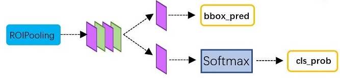
从PoI Pooling获取到7x7=49大小的proposal feature maps后,送入后续网络,可以看到做了如下2件事:
通过全连接和softmax对proposals进行分类,这实际上已经是识别的范畴了
再次对proposals进行bounding box regression,获取更高精度的rect box

Faster RCNN训练

Faster CNN的训练,是在已经训练好的model(如VGG_CNN_M_1024,VGG,ZF)的基础上继续进行训练。实际中训练过程分为6个步骤:
1.在已经训练好的model上,训练RPN网络,对应stage1_rpn_train.pt
2.利用步骤1中训练好的RPN网络,收集proposals,对应rpn_test.pt
3.第一次训练Fast RCNN网络,对应stage1_fast_rcnn_train.pt
4.第二训练RPN网络,对应stage2_rpn_train.pt
5.再次利用步骤4中训练好的RPN网络,收集proposals,对应rpn_test.pt
6.第二次训练Fast RCNN网络,对应stage2_fast_rcnn_train.pt

可以看到训练过程类似于一种“迭代”的过程,不过只循环了2次。至于只循环了2次的原因是应为作者提到:”A similar alternating training can be run for more iterations, but we have observed negligible improvements”,即循环更多次没有提升了。
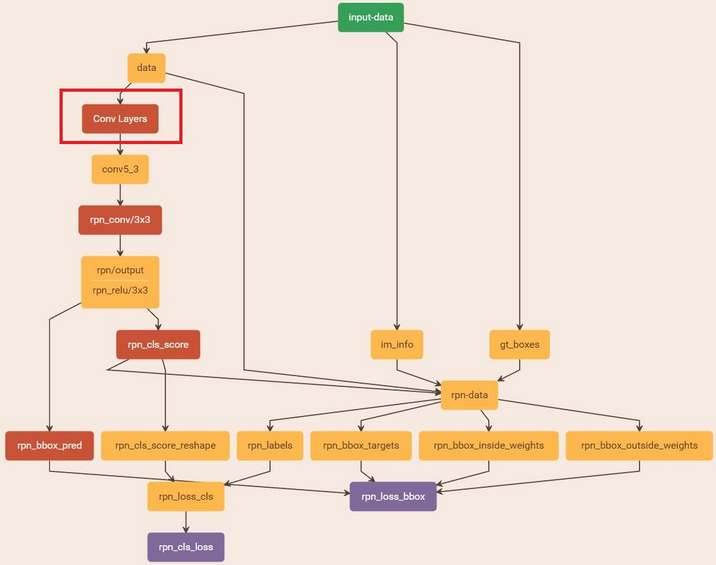
训练RPN网络

"da"

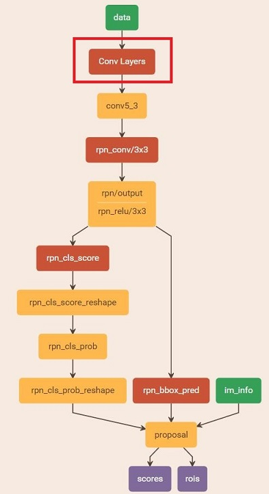
通过训练好的RPN网络收集proposals

在该步骤中,利用之前的RPN网络,获取proposal rois,同时获取foreground softmax probability,如下图,然后将获取的信息保存在python pickle文件中

"da"

整个网络使用的Loss如下

"da"

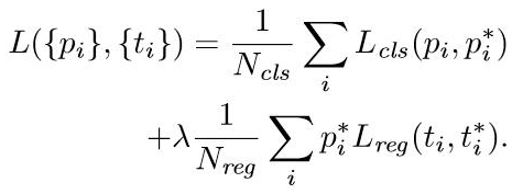
Ncls和Nreg差距过大,用参数λ平衡二者(如Ncls=256,Nreg=2400时设置λ=10)

训练Fast RCNN网络

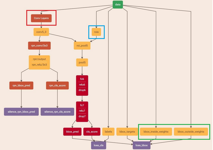
读取之前保存的pickle文件,获取proposals与foreground probability。从data层输入网络。然后:
将提取的proposals作为rois传入网络,如下图蓝框
将foreground probability作为bbox_inside_weights传入网络,如下图绿框
通过caffe blob大小对比,计算出bbox_outside_weights(即λ),如下图绿框

"da"

此外,Faster RCNN还有一种end-to-end的训练方式,可以一次完成train

-------------本文结束感谢您的阅读-------------